Unidad 4.3
dgonzalez

Pruebas paramétricas
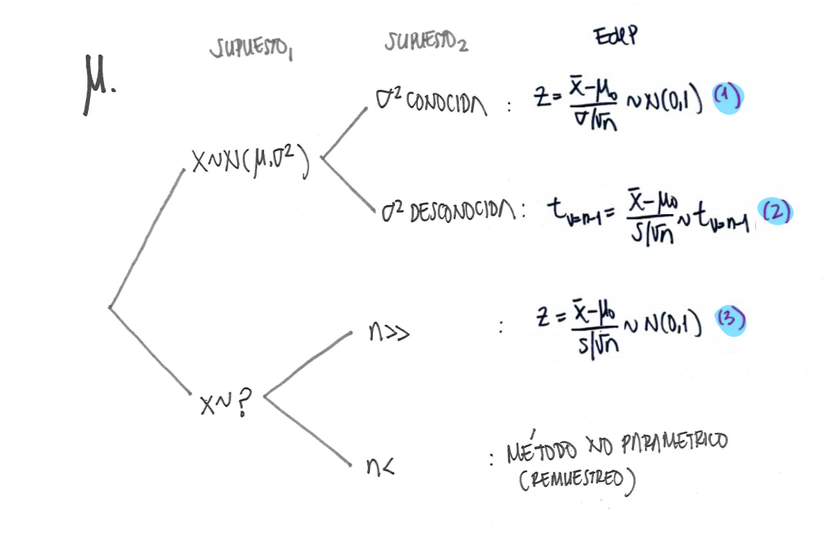
Pruebas de hipótesis sobre la media poblacional \(\mu\)
En el caso de las pruebas sobre la media poblacional se tienen las siguientes alternativas:
Supongamos las hipótesis de dos colas sobre una media:
| \(Ho\) : \(\mu_{W} = 1000\) |
| \(Ha\) : \(\mu_{W} \neq 1000\) |
En ella el investigador desea validar si la media poblacional \(\mu\) es diferente a 1000. Solo en caso de rechazar \(Ho\), podrá concluir que \(Ho\) es falsa y como consecuencia de ello \(Ha\) es verdad.
Antes de seleccionar el procedimiento a realizar, es necesario
validar en los datos si ellos siguen una distribución normal o no, pues
de ello depende la prueba apropiada que se debe realizar.
# Problema 1
w= round(rnorm(100,1000,5), 1) # simulación de los datos
w
[1] 998.8 1008.2 997.1 1002.0 1000.7 1011.9 1000.0 1003.9 994.1 994.6
[11] 1003.3 1004.4 999.0 1008.7 994.6 998.5 1005.1 997.8 1002.1 996.4
[21] 999.5 993.4 996.1 1004.4 1007.0 1006.5 987.6 992.3 1001.7 992.7
[31] 999.7 991.9 999.8 995.8 997.4 1000.8 999.1 1001.0 994.8 990.2
[41] 1002.4 1001.6 1006.2 995.5 991.1 1002.3 1000.5 1000.9 1000.9 1008.6
[51] 999.7 1002.9 1004.3 1007.0 999.7 991.4 998.6 1006.8 990.1 997.2
[61] 989.8 1000.7 994.8 997.2 1003.2 1002.6 1004.7 1006.2 994.7 992.6
[71] 995.3 999.0 996.9 1000.4 1003.4 998.8 1007.8 1004.2 1002.4 1002.9
[81] 1002.7 992.5 999.0 996.7 1004.8 999.0 1001.6 1000.6 999.2 996.6
[91] 1006.1 1000.1 1006.4 999.3 993.9 992.7 996.3 995.9 996.7 1002.9Realicemos entonces el siguiente contraste de hipótesis:
| \(Ho\) : \(X \sim norm\) |
| \(Ha\) : \(X no \sim norm\) |
shapiro.test(w) # verificación de normalidad
    Shapiro-Wilk normality test

data:  w
W = 0.99322, p-value = 0.901
Empleando la Regla 2
Si el valor-p < \(\alpha\), se rechaza \(Ho\), se acepta \(Ha\) como verdadera, de lo contrario no se rechaza \(Ho\), se asume que \(Ho\) es verdad.
Como el valor-p (0.323) < \(\alpha\) = 0.05, No se rechaza la hipótesis que los datos proceden de una distribución normal, asumimos que se distribuyen normal.
Caso con variable con distribución normal y varianza conocida
Supuestos:
| X normal |
| Varianza conocida (\(\sigma^{2}=4\)) |
BSDA::z.test(w, mu=1000, sigma.x = 2)
    One-sample z-Test

data:  w
z = -1.94, p-value = 0.05238
alternative hypothesis: true mean is not equal to 1000
95 percent confidence interval:
  999.220 1000.004
sample estimates:
mean of x
  999.612
Alternativas para el planteamiento de las hipótesis
Podemos realizar pruebas de:
| Dos colas | Cola superior | Cola inferior |
|---|---|---|
| \(Ho\) : \(\mu = \mu_o\) | \(Ho\) : \(\mu \leq \mu_o\) | \(Ho\) : \(\mu \geq \mu_o\) |
| \(Ha\) : \(\mu \neq \mu_o\) | \(Ha\) : \(\mu > \mu_o\) | \(Ha\) : \(\mu < \mu_o\) |
Supuestos:
| X normal |
| Varianza desconocida |
Cuando se afirma que la varianza es conocida, se tiene como base para esta afirmación que se ha realizado censo y como producto de conocer todos los valores de la variables se puede obtener el valor del parámetro.
En caso que los datos que tenemos para la varianza procedan de una muestra, el valor obtenido \(s^{2}\), correponde a una estimación de la varianza y diremos que la varianza no se conoce y que la estimamos mediante los valores de una muestra.
| \(Ho\) : \(\mu \geq 5\) |
| \(Ha\) : \(\mu < 5\) |
#-------------------------------------------------------------------------------
# Problema 2
t=c(4.21,5.55,3.02,5.13,4.77,2.34,5.42,4.50,6.10,3.80,5.12,6.46,6.19,3.79,3.54)
mean(t)
[1] 4.662667sd(t)[1] 1.210658t.test(t,mu=5, alternative="less")
    One Sample t-test

data:  t
t = -1.0792, df = 14, p-value = 0.1494
alternative hypothesis: true mean is less than 5
95 percent confidence interval:
     -Inf 5.213235
sample estimates:
mean of x
4.662667 | \(Ho\) : \(p \geq 5\) |
| \(Ha\) : \(p < 5\) |
#-------------------------------------------------------------------------------
#Problema 3
z=(24/40-.76)/(sqrt(.76*(1-.76)/40))

prop.test(24,40,0.76,alternative="less")
    1-sample proportions test with continuity correction

data:  24 out of 40, null probability 0.76
X-squared = 4.7711, df = 1, p-value = 0.01447
alternative hypothesis: true p is less than 0.76
95 percent confidence interval:
 0.0000000 0.7282033
sample estimates:
  p
0.6 | \(Ho\) : \(\mu_1 \geq \mu_2\) |
| \(Ha\) : \(\mu_1 < \mu_2\) |
#---------------------------------------------------------------------------------
# Problema 4
n1=36 ; mx1=6 ; sx1=4
n2=40 ; mx2=8.2; sx2=4.3

F=sx1^2/sx2^2
RdeRF=qf(c(0.025,0.975),35,39)

#t.test(x1,x2,mu=0, alternative = "less")
s2p=((n1-1)*sx1^2+(n2-1)*sx2^2)/(n1+n2-2)
sp=sqrt(s2p)
T4=(mx1-mx2)/(sp*sqrt(1/n1+1/n2))
RdeRT4=qt(0.05,(n1+n2-2))| \(Ho\) : \(\mu_{g1} \geq \mu_{g2}\) |
| \(Ha\) : \(\mu_{g1} < \mu_{g2}\) |
#-----------------------------------------------------------------------------------
# Problema 5
p5=3/40
z5=(p5-0.05)/sqrt(0.05*0.95/40)
#----------------------------------------------------------------------------------
# Problema 6
g1=c(75,76,74,80,72,798,76,73,72,75)
g2=c(86,78,86,84,81,79,78,84,88,80)
mean(g1);sd(g1)[1] 147.1[1] 228.715mean(g2);sd(g2)[1] 82.4[1] 3.657564var.test(g1,g2)
    F test to compare two variances

data:  g1 and g2
F = 3910.3, num df = 9, denom df = 9, p-value = 8.882e-15
alternative hypothesis: true ratio of variances is not equal to 1
95 percent confidence interval:
   971.2524 15742.6704
sample estimates:
ratio of variances
          3910.257
t.test(g1,g2)
    Welch Two Sample t-test

data:  g1 and g2
t = 0.89445, df = 9.0046, p-value = 0.3944
alternative hypothesis: true difference in means is not equal to 0
95 percent confidence interval:
 -98.92101 228.32101
sample estimates:
mean of x mean of y
147.1 82.4 | \(Ho\) : \(p_1 = p_2\) |
| \(Ha\) : \(p \neq p_2\) |
#---------------------------------------------------------------------------------
# Problema 7

n1=400 ;x1=80
n2=400 ; x2=88

prop.test(c(80,88),c(400,400))
    2-sample test for equality of proportions with continuity correction

data:  c(80, 88) out of c(400, 400)
X-squared = 0.3692, df = 1, p-value = 0.5434
alternative hypothesis: two.sided
95 percent confidence interval:
 -0.07893199  0.03893199
sample estimates:
prop 1 prop 2
0.20 0.22 | \(Ho\) : \(\mu_1 \geq \mu_2\) |
| \(Ha\) : \(\mu_1 < \mu_2\) |
#-----------------------------------------------------------------------------------
# Problema 8
x1=c(45,73,46,124,30,57,83,34,26,17)
x2=c(36,60,44,119,35,51,77,29,24,11)
d=x1-x2

mean(d)
[1] 4.9sd(d)[1] 4.72464t.test(x1,x2,paired = TRUE)
    Paired t-test

data:  x1 and x2
t = 3.2796, df = 9, p-value = 0.009535
alternative hypothesis: true mean difference is not equal to 0
95 percent confidence interval:
 1.520196 8.279804
sample estimates:
mean difference
4.9 | \(Ho\) : \(\mu_{pa} \geq \mu_{pd}\) |
| \(Ha\) : \(\mu_{pa} < \mu_{pd}\) |
#------------------------------------------------------------------------------------
#Problema 9

pa=c(104.5,89,84.5,106,90,96,79,90,85,76.5,91.5,82.5,100.5,89.5,121.5,72)
pd=c(98,85.5,85,103.5,88.5,95,79.5,90,82,76,89.5,81,99.5,86.5,115.5,70)
d=pa-pd
mean(d)
[1] 2.0625sd(d)[1] 2.032035t.test(pa,pd,paired = TRUE)
    Paired t-test

data:  pa and pd
t = 4.06, df = 15, p-value = 0.001026
alternative hypothesis: true mean difference is not equal to 0
95 percent confidence interval:
 0.9797049 3.1452951
sample estimates:
mean difference
2.0625 | Verificación de normalidad | Comparación de varianzas | Diferencia de medias |
|---|---|---|
| \(Ho\) : \(X_{g1} \sim norm\) | \(Ho\) : \(\sigma^{2}_{g1} = \sigma^{2}_{g2}\) | \(Ho\) : \(\mu_{g1} \geq \mu_{g2}\) |
| \(Ha\) : \(X_{g2} no \sim norm\) | \(Ha\) : \(\sigma^{2}_{g1} \neq \sigma^{2}_{g2}\) | \(Ha\) : \(\mu_{g1} < \mu_{g2}\) |
#-----------------------------------------------------------------------
# Problema 10
g1=c(37,19,21,35,16,4,0,12,63,25,12,15)
g2=c(24,42,18,15,0,9,10,20,22,13)

mean(g1);sd(g1)
[1] 21.58333[1] 17.01581mean(g2);sd(g2)[1] 17.3[1] 11.20565var.test(g1,g2)
    F test to compare two variances

data:  g1 and g2
F = 2.3058, num df = 11, denom df = 9, p-value = 0.22
alternative hypothesis: true ratio of variances is not equal to 1
95 percent confidence interval:
 0.5894187 8.2731556
sample estimates:
ratio of variances
           2.30585
t.test(g1,g2)
    Welch Two Sample t-test

data:  g1 and g2
t = 0.70719, df = 19.104, p-value = 0.488
alternative hypothesis: true difference in means is not equal to 0
95 percent confidence interval:
 -8.389007 16.955673
sample estimates:
mean of x mean of y
 21.58333  17.30000
Pruebas no paramétricas
Prueba de rachas
library(randtests)
x=c("N","D","N","N","N","N","N","D","D","D","N","N","N","N","D","N","N","D","N","N","N","D","N","N","N","N","N","N","N","D","D","D","D")
rachas<-as.numeric(x=="N")
runs.test(rachas,alternative = "left.sided",threshold = 0.5,pvalue = "exact",plot=F)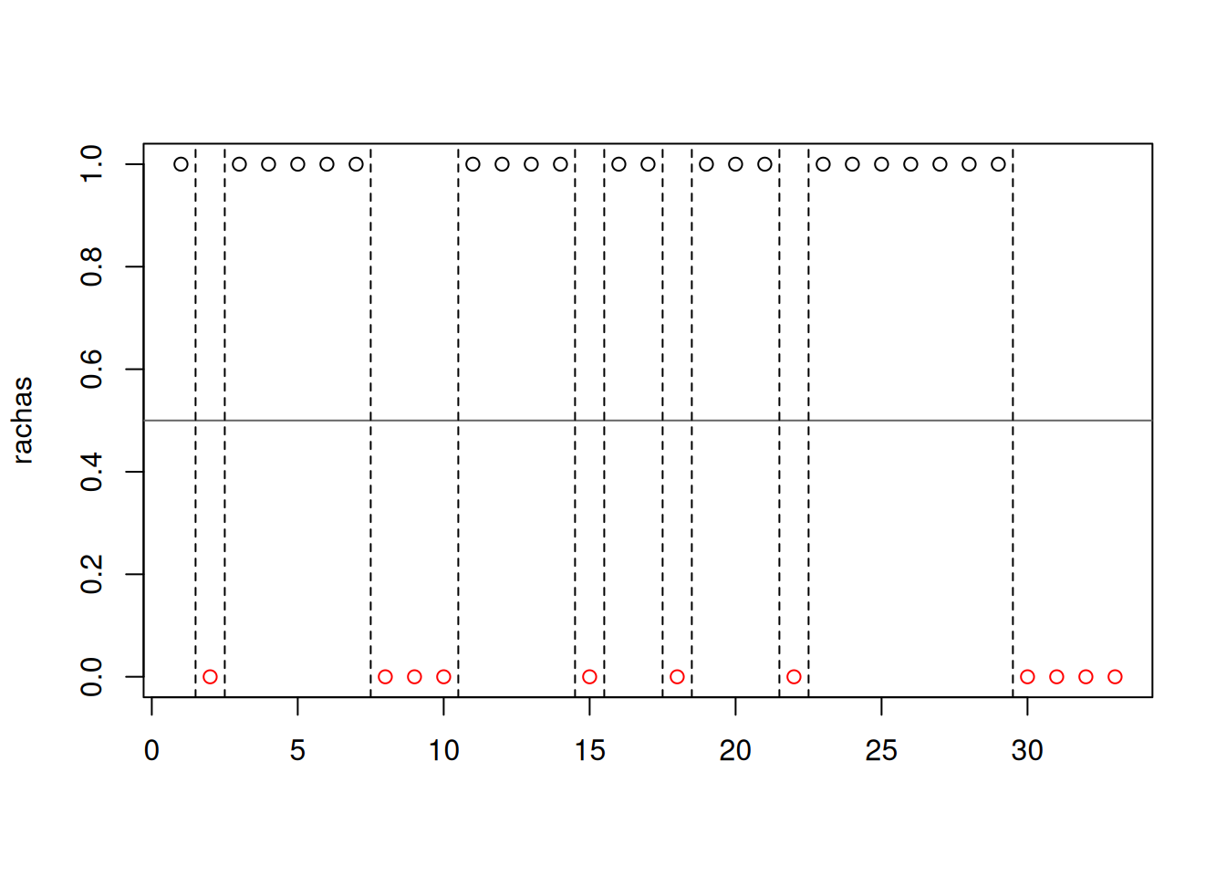
    Runs Test

data:  rachas
statistic = -1.465, runs = 12, n1 = 22, n2 = 11, n = 33, p-value =
0.1032
alternative hypothesis: trend
Pruebas de normalidad
Existen varias pruebas de hipótesis para verificar si una variable tiene un comportamiento aproximadamente normal.En todos los casos las hipótesis planteadas son:
| \(Ho\): \(X\) tiene distribución Normal |
| \(Ha\): \(X\) no tiene distribución Normal |
# se genera una variable aleatoria normal
# x=rnorm(100,1000,50) #round(x,1)
x <- c(946.5,  997.7, 1014.0, 1050.1,  942.3,  974.0,  997.4, 1135.8,  863.9, 1068.8,  956.9,  998.1,  997.6, 1023.4, 1008.7,  965.5,  974.8, 1063.6, 1001.2, 1090.9,  979.0,  931.5, 1018.7,  988.0,  979.9, 1043.0,  976.4, 1035.5, 1119.3,  924.3,  998.8, 1068.6,  975.5, 1037.1,  896.6,  954.7, 1029.4,  979.4,  984.1, 1004.2, 1075.1,  989.8, 1095.6, 1016.8,  909.6,  979.6, 1055.2, 1008.4, 1064.6,  994.1,  931.9,  910.8, 1045.9,  949.1, 1078.2, 1051.5,  946.9,  981.8,  988.1, 1007.5, 1082.1,  974.1, 1015.4,  961.6,  920.8,  938.1, 1008.1,  974.6, 1052.0,  986.1, 1042.3, 1014.5,  999.5,  962.0, 1024.0, 1012.4, 1014.8, 1038.4, 1084.1,  976.1,  916.2, 1023.4,  950.3, 1005.3,  945.2,  968.0, 1039.8, 1001.8,  964.4,  940.0,  982.5, 1012.9,  978.1, 1014.9,  999.0, 1031.3, 1025.6, 1034.4, 973.5, 1091.0)


plot(density(x), las=1)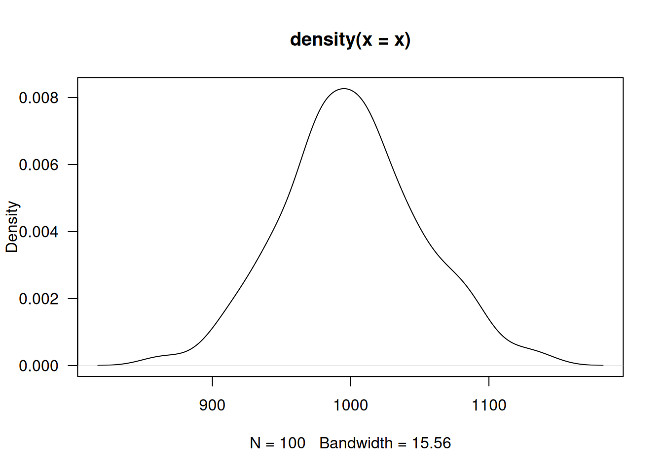
Shapiro Wilk
x <- c(946.5,  997.7, 1014.0, 1050.1,  942.3,  974.0,  997.4, 1135.8,  863.9, 1068.8,  956.9,  998.1,  997.6, 1023.4, 1008.7,  965.5,  974.8, 1063.6, 1001.2, 1090.9,  979.0,  931.5, 1018.7,  988.0,  979.9, 1043.0,  976.4, 1035.5, 1119.3,  924.3,  998.8, 1068.6,  975.5, 1037.1,  896.6,  954.7, 1029.4,  979.4,  984.1, 1004.2, 1075.1,  989.8, 1095.6, 1016.8,  909.6,  979.6, 1055.2, 1008.4, 1064.6,  994.1,  931.9,  910.8, 1045.9,  949.1, 1078.2, 1051.5,  946.9,  981.8,  988.1, 1007.5, 1082.1,  974.1, 1015.4,  961.6,  920.8,  938.1, 1008.1,  974.6, 1052.0,  986.1, 1042.3, 1014.5,  999.5,  962.0, 1024.0, 1012.4, 1014.8, 1038.4, 1084.1,  976.1,  916.2, 1023.4,  950.3, 1005.3,  945.2,  968.0, 1039.8, 1001.8,  964.4,  940.0,  982.5, 1012.9,  978.1, 1014.9,  999.0, 1031.3, 1025.6, 1034.4, 973.5, 1091.0)

shapiro.test(x)
    Shapiro-Wilk normality test

data:  x
W = 0.9956, p-value = 0.9877
Esta prueba no requiere la instalación de paquetes adicionales, está disponible en la configuración básica de R
Paquete normtest
Las siguientes pruebas requieren instalar y cargar el paquete:
normtest
# install.packages("normtets")
# library(normtest)
Jarque-Bera ajustado
x <- c(946.5,  997.7, 1014.0, 1050.1,  942.3,  974.0,  997.4, 1135.8,  863.9, 1068.8,  956.9,  998.1,  997.6, 1023.4, 1008.7,  965.5,  974.8, 1063.6, 1001.2, 1090.9,  979.0,  931.5, 1018.7,  988.0,  979.9, 1043.0,  976.4, 1035.5, 1119.3,  924.3,  998.8, 1068.6,  975.5, 1037.1,  896.6,  954.7, 1029.4,  979.4,  984.1, 1004.2, 1075.1,  989.8, 1095.6, 1016.8,  909.6,  979.6, 1055.2, 1008.4, 1064.6,  994.1,  931.9,  910.8, 1045.9,  949.1, 1078.2, 1051.5,  946.9,  981.8,  988.1, 1007.5, 1082.1,  974.1, 1015.4,  961.6,  920.8,  938.1, 1008.1,  974.6, 1052.0,  986.1, 1042.3, 1014.5,  999.5,  962.0, 1024.0, 1012.4, 1014.8, 1038.4, 1084.1,  976.1,  916.2, 1023.4,  950.3, 1005.3,  945.2,  968.0, 1039.8, 1001.8,  964.4,  940.0,  982.5, 1012.9,  978.1, 1014.9,  999.0, 1031.3, 1025.6, 1034.4, 973.5, 1091.0)

ajb.norm.test(x)
Frosini
x <- c(946.5,  997.7, 1014.0, 1050.1,  942.3,  974.0,  997.4, 1135.8,  863.9, 1068.8,  956.9,  998.1,  997.6, 1023.4, 1008.7,  965.5,  974.8, 1063.6, 1001.2, 1090.9,  979.0,  931.5, 1018.7,  988.0,  979.9, 1043.0,  976.4, 1035.5, 1119.3,  924.3,  998.8, 1068.6,  975.5, 1037.1,  896.6,  954.7, 1029.4,  979.4,  984.1, 1004.2, 1075.1,  989.8, 1095.6, 1016.8,  909.6,  979.6, 1055.2, 1008.4, 1064.6,  994.1,  931.9,  910.8, 1045.9,  949.1, 1078.2, 1051.5,  946.9,  981.8,  988.1, 1007.5, 1082.1,  974.1, 1015.4,  961.6,  920.8,  938.1, 1008.1,  974.6, 1052.0,  986.1, 1042.3, 1014.5,  999.5,  962.0, 1024.0, 1012.4, 1014.8, 1038.4, 1084.1,  976.1,  916.2, 1023.4,  950.3, 1005.3,  945.2,  968.0, 1039.8, 1001.8,  964.4,  940.0,  982.5, 1012.9,  978.1, 1014.9,  999.0, 1031.3, 1025.6, 1034.4, 973.5, 1091.0)

frosini.norm.test(x)
Geary
x <- c(946.5,  997.7, 1014.0, 1050.1,  942.3,  974.0,  997.4, 1135.8,  863.9, 1068.8,  956.9,  998.1,  997.6, 1023.4, 1008.7,  965.5,  974.8, 1063.6, 1001.2, 1090.9,  979.0,  931.5, 1018.7,  988.0,  979.9, 1043.0,  976.4, 1035.5, 1119.3,  924.3,  998.8, 1068.6,  975.5, 1037.1,  896.6,  954.7, 1029.4,  979.4,  984.1, 1004.2, 1075.1,  989.8, 1095.6, 1016.8,  909.6,  979.6, 1055.2, 1008.4, 1064.6,  994.1,  931.9,  910.8, 1045.9,  949.1, 1078.2, 1051.5,  946.9,  981.8,  988.1, 1007.5, 1082.1,  974.1, 1015.4,  961.6,  920.8,  938.1, 1008.1,  974.6, 1052.0,  986.1, 1042.3, 1014.5,  999.5,  962.0, 1024.0, 1012.4, 1014.8, 1038.4, 1084.1,  976.1,  916.2, 1023.4,  950.3, 1005.3,  945.2,  968.0, 1039.8, 1001.8,  964.4,  940.0,  982.5, 1012.9,  978.1, 1014.9,  999.0, 1031.3, 1025.6, 1034.4, 973.5, 1091.0)


geary.norm.test(x)
Hagazy-Green 1
x <- c(946.5,  997.7, 1014.0, 1050.1,  942.3,  974.0,  997.4, 1135.8,  863.9, 1068.8,  956.9,  998.1,  997.6, 1023.4, 1008.7,  965.5,  974.8, 1063.6, 1001.2, 1090.9,  979.0,  931.5, 1018.7,  988.0,  979.9, 1043.0,  976.4, 1035.5, 1119.3,  924.3,  998.8, 1068.6,  975.5, 1037.1,  896.6,  954.7, 1029.4,  979.4,  984.1, 1004.2, 1075.1,  989.8, 1095.6, 1016.8,  909.6,  979.6, 1055.2, 1008.4, 1064.6,  994.1,  931.9,  910.8, 1045.9,  949.1, 1078.2, 1051.5,  946.9,  981.8,  988.1, 1007.5, 1082.1,  974.1, 1015.4,  961.6,  920.8,  938.1, 1008.1,  974.6, 1052.0,  986.1, 1042.3, 1014.5,  999.5,  962.0, 1024.0, 1012.4, 1014.8, 1038.4, 1084.1,  976.1,  916.2, 1023.4,  950.3, 1005.3,  945.2,  968.0, 1039.8, 1001.8,  964.4,  940.0,  982.5, 1012.9,  978.1, 1014.9,  999.0, 1031.3, 1025.6, 1034.4, 973.5, 1091.0)


hegazy1.norm.test(x)
Hagazy-Green 2
x <- c(946.5,  997.7, 1014.0, 1050.1,  942.3,  974.0,  997.4, 1135.8,  863.9, 1068.8,  956.9,  998.1,  997.6, 1023.4, 1008.7,  965.5,  974.8, 1063.6, 1001.2, 1090.9,  979.0,  931.5, 1018.7,  988.0,  979.9, 1043.0,  976.4, 1035.5, 1119.3,  924.3,  998.8, 1068.6,  975.5, 1037.1,  896.6,  954.7, 1029.4,  979.4,  984.1, 1004.2, 1075.1,  989.8, 1095.6, 1016.8,  909.6,  979.6, 1055.2, 1008.4, 1064.6,  994.1,  931.9,  910.8, 1045.9,  949.1, 1078.2, 1051.5,  946.9,  981.8,  988.1, 1007.5, 1082.1,  974.1, 1015.4,  961.6,  920.8,  938.1, 1008.1,  974.6, 1052.0,  986.1, 1042.3, 1014.5,  999.5,  962.0, 1024.0, 1012.4, 1014.8, 1038.4, 1084.1,  976.1,  916.2, 1023.4,  950.3, 1005.3,  945.2,  968.0, 1039.8, 1001.8,  964.4,  940.0,  982.5, 1012.9,  978.1, 1014.9,  999.0, 1031.3, 1025.6, 1034.4, 973.5, 1091.0)

hegazy2.norm.test(x)
Jarque-Bera
x <- c(946.5,  997.7, 1014.0, 1050.1,  942.3,  974.0,  997.4, 1135.8,  863.9, 1068.8,  956.9,  998.1,  997.6, 1023.4, 1008.7,  965.5,  974.8, 1063.6, 1001.2, 1090.9,  979.0,  931.5, 1018.7,  988.0,  979.9, 1043.0,  976.4, 1035.5, 1119.3,  924.3,  998.8, 1068.6,  975.5, 1037.1,  896.6,  954.7, 1029.4,  979.4,  984.1, 1004.2, 1075.1,  989.8, 1095.6, 1016.8,  909.6,  979.6, 1055.2, 1008.4, 1064.6,  994.1,  931.9,  910.8, 1045.9,  949.1, 1078.2, 1051.5,  946.9,  981.8,  988.1, 1007.5, 1082.1,  974.1, 1015.4,  961.6,  920.8,  938.1, 1008.1,  974.6, 1052.0,  986.1, 1042.3, 1014.5,  999.5,  962.0, 1024.0, 1012.4, 1014.8, 1038.4, 1084.1,  976.1,  916.2, 1023.4,  950.3, 1005.3,  945.2,  968.0, 1039.8, 1001.8,  964.4,  940.0,  982.5, 1012.9,  978.1, 1014.9,  999.0, 1031.3, 1025.6, 1034.4, 973.5, 1091.0)

jb.norm.test(x)
de kurtosis
x <- c(946.5,  997.7, 1014.0, 1050.1,  942.3,  974.0,  997.4, 1135.8,  863.9, 1068.8,  956.9,  998.1,  997.6, 1023.4, 1008.7,  965.5,  974.8, 1063.6, 1001.2, 1090.9,  979.0,  931.5, 1018.7,  988.0,  979.9, 1043.0,  976.4, 1035.5, 1119.3,  924.3,  998.8, 1068.6,  975.5, 1037.1,  896.6,  954.7, 1029.4,  979.4,  984.1, 1004.2, 1075.1,  989.8, 1095.6, 1016.8,  909.6,  979.6, 1055.2, 1008.4, 1064.6,  994.1,  931.9,  910.8, 1045.9,  949.1, 1078.2, 1051.5,  946.9,  981.8,  988.1, 1007.5, 1082.1,  974.1, 1015.4,  961.6,  920.8,  938.1, 1008.1,  974.6, 1052.0,  986.1, 1042.3, 1014.5,  999.5,  962.0, 1024.0, 1012.4, 1014.8, 1038.4, 1084.1,  976.1,  916.2, 1023.4,  950.3, 1005.3,  945.2,  968.0, 1039.8, 1001.8,  964.4,  940.0,  982.5, 1012.9,  978.1, 1014.9,  999.0, 1031.3, 1025.6, 1034.4, 973.5, 1091.0)


kurtosis.norm.test(x)
de sesgo
x <- c(946.5,  997.7, 1014.0, 1050.1,  942.3,  974.0,  997.4, 1135.8,  863.9, 1068.8,  956.9,  998.1,  997.6, 1023.4, 1008.7,  965.5,  974.8, 1063.6, 1001.2, 1090.9,  979.0,  931.5, 1018.7,  988.0,  979.9, 1043.0,  976.4, 1035.5, 1119.3,  924.3,  998.8, 1068.6,  975.5, 1037.1,  896.6,  954.7, 1029.4,  979.4,  984.1, 1004.2, 1075.1,  989.8, 1095.6, 1016.8,  909.6,  979.6, 1055.2, 1008.4, 1064.6,  994.1,  931.9,  910.8, 1045.9,  949.1, 1078.2, 1051.5,  946.9,  981.8,  988.1, 1007.5, 1082.1,  974.1, 1015.4,  961.6,  920.8,  938.1, 1008.1,  974.6, 1052.0,  986.1, 1042.3, 1014.5,  999.5,  962.0, 1024.0, 1012.4, 1014.8, 1038.4, 1084.1,  976.1,  916.2, 1023.4,  950.3, 1005.3,  945.2,  968.0, 1039.8, 1001.8,  964.4,  940.0,  982.5, 1012.9,  978.1, 1014.9,  999.0, 1031.3, 1025.6, 1034.4, 973.5, 1091.0)

skewness.norm.test(x)
Spiegelhalter
x <- c(946.5,  997.7, 1014.0, 1050.1,  942.3,  974.0,  997.4, 1135.8,  863.9, 1068.8,  956.9,  998.1,  997.6, 1023.4, 1008.7,  965.5,  974.8, 1063.6, 1001.2, 1090.9,  979.0,  931.5, 1018.7,  988.0,  979.9, 1043.0,  976.4, 1035.5, 1119.3,  924.3,  998.8, 1068.6,  975.5, 1037.1,  896.6,  954.7, 1029.4,  979.4,  984.1, 1004.2, 1075.1,  989.8, 1095.6, 1016.8,  909.6,  979.6, 1055.2, 1008.4, 1064.6,  994.1,  931.9,  910.8, 1045.9,  949.1, 1078.2, 1051.5,  946.9,  981.8,  988.1, 1007.5, 1082.1,  974.1, 1015.4,  961.6,  920.8,  938.1, 1008.1,  974.6, 1052.0,  986.1, 1042.3, 1014.5,  999.5,  962.0, 1024.0, 1012.4, 1014.8, 1038.4, 1084.1,  976.1,  916.2, 1023.4,  950.3, 1005.3,  945.2,  968.0, 1039.8, 1001.8,  964.4,  940.0,  982.5, 1012.9,  978.1, 1014.9,  999.0, 1031.3, 1025.6, 1034.4, 973.5, 1091.0)


spiegelhalter.norm.test(x)
Weisberg-Bingham
x <- c(946.5,  997.7, 1014.0, 1050.1,  942.3,  974.0,  997.4, 1135.8,  863.9, 1068.8,  956.9,  998.1,  997.6, 1023.4, 1008.7,  965.5,  974.8, 1063.6, 1001.2, 1090.9,  979.0,  931.5, 1018.7,  988.0,  979.9, 1043.0,  976.4, 1035.5, 1119.3,  924.3,  998.8, 1068.6,  975.5, 1037.1,  896.6,  954.7, 1029.4,  979.4,  984.1, 1004.2, 1075.1,  989.8, 1095.6, 1016.8,  909.6,  979.6, 1055.2, 1008.4, 1064.6,  994.1,  931.9,  910.8, 1045.9,  949.1, 1078.2, 1051.5,  946.9,  981.8,  988.1, 1007.5, 1082.1,  974.1, 1015.4,  961.6,  920.8,  938.1, 1008.1,  974.6, 1052.0,  986.1, 1042.3, 1014.5,  999.5,  962.0, 1024.0, 1012.4, 1014.8, 1038.4, 1084.1,  976.1,  916.2, 1023.4,  950.3, 1005.3,  945.2,  968.0, 1039.8, 1001.8,  964.4,  940.0,  982.5, 1012.9,  978.1, 1014.9,  999.0, 1031.3, 1025.6, 1034.4, 973.5, 1091.0)

wb.norm.test(x)
Paquete nortest
Las siguientes pruebas requieren instalar y cargar el paquete:
nortest
# install.packages("nortets")
library(nortest)
Anderson-Darling
x <- c(946.5,  997.7, 1014.0, 1050.1,  942.3,  974.0,  997.4, 1135.8,  863.9, 1068.8,  956.9,  998.1,  997.6, 1023.4, 1008.7,  965.5,  974.8, 1063.6, 1001.2, 1090.9,  979.0,  931.5, 1018.7,  988.0,  979.9, 1043.0,  976.4, 1035.5, 1119.3,  924.3,  998.8, 1068.6,  975.5, 1037.1,  896.6,  954.7, 1029.4,  979.4,  984.1, 1004.2, 1075.1,  989.8, 1095.6, 1016.8,  909.6,  979.6, 1055.2, 1008.4, 1064.6,  994.1,  931.9,  910.8, 1045.9,  949.1, 1078.2, 1051.5,  946.9,  981.8,  988.1, 1007.5, 1082.1,  974.1, 1015.4,  961.6,  920.8,  938.1, 1008.1,  974.6, 1052.0,  986.1, 1042.3, 1014.5,  999.5,  962.0, 1024.0, 1012.4, 1014.8, 1038.4, 1084.1,  976.1,  916.2, 1023.4,  950.3, 1005.3,  945.2,  968.0, 1039.8, 1001.8,  964.4,  940.0,  982.5, 1012.9,  978.1, 1014.9,  999.0, 1031.3, 1025.6, 1034.4, 973.5, 1091.0)

ad.test(x)
    Anderson-Darling normality test

data:  x
A = 0.20586, p-value = 0.8673
Cramer-von Mises
x <- c(946.5,  997.7, 1014.0, 1050.1,  942.3,  974.0,  997.4, 1135.8,  863.9, 1068.8,  956.9,  998.1,  997.6, 1023.4, 1008.7,  965.5,  974.8, 1063.6, 1001.2, 1090.9,  979.0,  931.5, 1018.7,  988.0,  979.9, 1043.0,  976.4, 1035.5, 1119.3,  924.3,  998.8, 1068.6,  975.5, 1037.1,  896.6,  954.7, 1029.4,  979.4,  984.1, 1004.2, 1075.1,  989.8, 1095.6, 1016.8,  909.6,  979.6, 1055.2, 1008.4, 1064.6,  994.1,  931.9,  910.8, 1045.9,  949.1, 1078.2, 1051.5,  946.9,  981.8,  988.1, 1007.5, 1082.1,  974.1, 1015.4,  961.6,  920.8,  938.1, 1008.1,  974.6, 1052.0,  986.1, 1042.3, 1014.5,  999.5,  962.0, 1024.0, 1012.4, 1014.8, 1038.4, 1084.1,  976.1,  916.2, 1023.4,  950.3, 1005.3,  945.2,  968.0, 1039.8, 1001.8,  964.4,  940.0,  982.5, 1012.9,  978.1, 1014.9,  999.0, 1031.3, 1025.6, 1034.4, 973.5, 1091.0)

cvm.test(x)
    Cramer-von Mises normality test

data:  x
W = 0.037008, p-value = 0.7332
Lilliefors (Kolmogorov-Smirnov)
x <- c(946.5,  997.7, 1014.0, 1050.1,  942.3,  974.0,  997.4, 1135.8,  863.9, 1068.8,  956.9,  998.1,  997.6, 1023.4, 1008.7,  965.5,  974.8, 1063.6, 1001.2, 1090.9,  979.0,  931.5, 1018.7,  988.0,  979.9, 1043.0,  976.4, 1035.5, 1119.3,  924.3,  998.8, 1068.6,  975.5, 1037.1,  896.6,  954.7, 1029.4,  979.4,  984.1, 1004.2, 1075.1,  989.8, 1095.6, 1016.8,  909.6,  979.6, 1055.2, 1008.4, 1064.6,  994.1,  931.9,  910.8, 1045.9,  949.1, 1078.2, 1051.5,  946.9,  981.8,  988.1, 1007.5, 1082.1,  974.1, 1015.4,  961.6,  920.8,  938.1, 1008.1,  974.6, 1052.0,  986.1, 1042.3, 1014.5,  999.5,  962.0, 1024.0, 1012.4, 1014.8, 1038.4, 1084.1,  976.1,  916.2, 1023.4,  950.3, 1005.3,  945.2,  968.0, 1039.8, 1001.8,  964.4,  940.0,  982.5, 1012.9,  978.1, 1014.9,  999.0, 1031.3, 1025.6, 1034.4, 973.5, 1091.0)

lillie.test(x)
    Lilliefors (Kolmogorov-Smirnov) normality test

data:  x
D = 0.054822, p-value = 0.6495
chi-cuadrado de Pearson
x <- c(946.5,  997.7, 1014.0, 1050.1,  942.3,  974.0,  997.4, 1135.8,  863.9, 1068.8,  956.9,  998.1,  997.6, 1023.4, 1008.7,  965.5,  974.8, 1063.6, 1001.2, 1090.9,  979.0,  931.5, 1018.7,  988.0,  979.9, 1043.0,  976.4, 1035.5, 1119.3,  924.3,  998.8, 1068.6,  975.5, 1037.1,  896.6,  954.7, 1029.4,  979.4,  984.1, 1004.2, 1075.1,  989.8, 1095.6, 1016.8,  909.6,  979.6, 1055.2, 1008.4, 1064.6,  994.1,  931.9,  910.8, 1045.9,  949.1, 1078.2, 1051.5,  946.9,  981.8,  988.1, 1007.5, 1082.1,  974.1, 1015.4,  961.6,  920.8,  938.1, 1008.1,  974.6, 1052.0,  986.1, 1042.3, 1014.5,  999.5,  962.0, 1024.0, 1012.4, 1014.8, 1038.4, 1084.1,  976.1,  916.2, 1023.4,  950.3, 1005.3,  945.2,  968.0, 1039.8, 1001.8,  964.4,  940.0,  982.5, 1012.9,  978.1, 1014.9,  999.0, 1031.3, 1025.6, 1034.4, 973.5, 1091.0)

pearson.test(x)
    Pearson chi-square normality test

data:  x
P = 7.38, p-value = 0.6891
Shapiro-Francia
x <- c(946.5,  997.7, 1014.0, 1050.1,  942.3,  974.0,  997.4, 1135.8,  863.9, 1068.8,  956.9,  998.1,  997.6, 1023.4, 1008.7,  965.5,  974.8, 1063.6, 1001.2, 1090.9,  979.0,  931.5, 1018.7,  988.0,  979.9, 1043.0,  976.4, 1035.5, 1119.3,  924.3,  998.8, 1068.6,  975.5, 1037.1,  896.6,  954.7, 1029.4,  979.4,  984.1, 1004.2, 1075.1,  989.8, 1095.6, 1016.8,  909.6,  979.6, 1055.2, 1008.4, 1064.6,  994.1,  931.9,  910.8, 1045.9,  949.1, 1078.2, 1051.5,  946.9,  981.8,  988.1, 1007.5, 1082.1,  974.1, 1015.4,  961.6,  920.8,  938.1, 1008.1,  974.6, 1052.0,  986.1, 1042.3, 1014.5,  999.5,  962.0, 1024.0, 1012.4, 1014.8, 1038.4, 1084.1,  976.1,  916.2, 1023.4,  950.3, 1005.3,  945.2,  968.0, 1039.8, 1001.8,  964.4,  940.0,  982.5, 1012.9,  978.1, 1014.9,  999.0, 1031.3, 1025.6, 1034.4, 973.5, 1091.0)

sf.test(x)
    Shapiro-Francia normality test

data:  x
W = 0.99466, p-value = 0.923
En todos los casos se presenta un valor-p grande por lo cual no se rechaza \(Ho\), asumimos que \(Ho\) es verdad. Asumimos que la distribución de la variable \(X\) es normal
Referencias :